Quadratic forms, local minimizers, and a cool relationship between the two

This semester, I am diverging a bit from the usual Aerospace Engineering workload with a math class that I had been eyeing for a while: MATH 467, Theory and Computational Methods of Optimization. It is no surprise that this interests me - half of designing airplanes is optimizing them, and I’ve found a great passion in modelling/simulations for trade studies and design space investigations in the early conceptual design phase.

What I underestimated is the “MATH” part of “MATH 467.” This course is quite theory heavy, with a less pronounced “computational” part as I had hoped for. However, I’ve been having an awful lot of fun, and sometime ago a friend and I had a small lightbulb moment that I thought I’d share. It is not much per se, just a cool little insight. But first, a bit of linear algebra…

Quadratic Forms

During the first couple of weeks, the class was a review of linear algebra. This has become the subject that fascinates me the most: even the most simple definitions have geometric interpretations that give a lot of insight into other areas of the subject. We reviewed one thing, however, that I had never come across before: quadratic forms.

A quadratic form is simply a function $f:\mathbb{R}^n\rightarrow\mathbb{R}$ of the form:

$$f(x)=x^TQx$$

Where $Q\in\mathbb{R}^{nxn}$ is a symmetric matrix. Note the domain and range in the function here: $f$ takes in a vector $x\in\mathbb{R}^n$ and outputs a real number $f(x)\in\mathbb{R}$.

These are called quadratic forms because the polynomial $f(x)$ will be of second degree. More accurately, the polynomial itself is in quadratic form, and it just so happens that we can write it in the form $x^TQx$ for a symmetric matrix $Q$.

Another quadratic form fun fact: there is no loss of generality in demanding that $Q$ be symmetric, because you can always let:

$$\widetilde{Q}=\frac{1}{2}\left(Q+Q^T\right)$$

Which guarantees $\widetilde{Q}=\widetilde{Q}^T$ and:

$$f(x)=x^T\widetilde{Q}x=x^TQx=x^T\left(\frac{1}{2}Q+\frac{1}{2}Q^T\right)x$$

A simple example in 3D gives some more insight into what this truly means. Consider the matrix $A\in\mathbb{R}^{3}$:

$$A = \begin{bmatrix}a_{11}&a_{12}&a_{13}\\a_{21}&a_{22}&a_{23}\\a_{31}&a_{32}&a_{33}\end{bmatrix}$$

We can find its quadratic form simply by the definition:

$$f(x)=\begin{bmatrix}x_1&x_2&x_3\end{bmatrix}\begin{bmatrix}a_{11}&a_{12}&a_{13}\\a_{21}&a_{22}&a_{23}\\a_{31}&a_{32}&a_{33}\end{bmatrix}\begin{bmatrix}x_1\\x_2\\x_3\end{bmatrix}$$

Multiplying these out yields:

$$f(x)=a_{11}x_1^2+a_{22}x_2^2+a_{33}x_3^2\\+(a_{12}+a_{21})x_1x_2+(a_{13}+a_{31})x_1x_3+(a_{23}+a_{32})x_2x_3$$

We thus see that the matrix $A$ simply holds the coefficients to the quadratic polynomial $f(x)$! It also becomes clear why there is no loss of generality when we take the “average” matrix, that is, half of the sum of the matrix and its transpose. The new matrix will have equal diagonal (since the transpose’s diagonal doesn’t change, and adding then halving the same entries will just give us the original entries.) The “cross” terms, that is, $a_{i,j}$ when $i\neq j$, will be added together and halved. However, their sum appears in the quadratic expansion. Take the $x_1x_3$ term, for example:

$$(a_{13,\widetilde{Q}}+a_{31\widetilde{Q}})x_1x_3=\frac{1}{2}(a_{13}+a_{31}+a_{31}+a_{13})x_1x_3=(a_{13}+a_{31})x_1x_3$$

So the quadratic form is preserved.

At this point, I thought to myself: “cool.” But also… where is this used? Turning to my friend and asking this question, he said “apparently everywhere.” And he was right! Quadratic forms are incredibly important in statistics, mechanics, and many other areas of mathematics. For the purpose of this class, they are also incredibly important: they show up all the time in optimization. This post will explore one example of such appearance.

But first, another concept that is almost equally important to the quadratic form itself: its definiteness.

Definiteness of a Quadratic Form

A quadratic form can be deemed positive definite, positive semidefinite, negative definite, or negative semidefinite.

A quadratic form is positive definite if:

$$f(x)=x^TQx>0\ \forall \ x\ne0$$

And it is positive semidefinite if:

$$f(x)=x^TQx\ge 0\ \forall \ x\in\mathbb{R}^n$$

In words: f is positive definite if it is positive for all nonzero vectors $x$, and positive semidefinite if it is positive or zero for all vectors $x$. Negative definite and semidefinite forms are defined similarly (in terms of the strict inequality and nullity or otherwise of possible $x$.)

There is a nice method for determining whether the quadratic form of a matrix is positive definite called Sylvester’s Criterion. It states that A matrix is positive definite if and only if all of its leading principal minors are nonnegative.

This was another new one to me - what are leading principal minors? The definition might seem loose but is visually pretty satisfying: these are the determinants of the matrices obtained by successively removing the last row and column.

Back to our $\mathbb{R}^{3x3}$ example:

$$A = \begin{bmatrix}a_{11}&a_{12}&a_{13}\\a_{21}&a_{22}&a_{23}\\a_{31}&a_{32}&a_{33}\end{bmatrix}$$

Let’s successively remove the last rows and columns, and let’s call these submatrices $A_n$. Before we even begin, the determinant of matrix $A$ itself is a minor:

$$\det(A_0) = \begin{vmatrix}a_{11}&a_{12}&a_{13}\\a_{21}&a_{22}&a_{23}\\a_{31}&a_{32}&a_{33}\end{vmatrix}$$

Removing the last row and column, we get the next minor:

$$\det(A_1) = \begin{vmatrix}a_{11}&a_{12}\\a_{21}&a_{22}\end{vmatrix}$$

Removing the last row and column, we get the last minor:

$$\det(A_2) = \begin{vmatrix}a_{11}\end{vmatrix}$$

Which is, of course, just $a_{11}$. From Sylvester’s Criterion, therefore, $A$ is positive definite if and only if:

$$\det(A_0)\geq0,\det(A_1)\geq0,\det(A_2)\geq0$$

This can come in quite handy!

Ok, before we talk about minimizers, there is one last thing to be introduced.

Multivariate Taylor Expansion

For a single variable function .$f:\mathbb{R}\rightarrow\mathbb{R}$, the Taylor expansion about $a$ is the very familiar polynomial:

$$f(x)=f(a)+f'(a)(x-a)+\frac{1}{2!}f''(a)(x-a)^2+\frac{1}{3!}f^{(3)}(a)(x-a)^3...$$

However, we now want to consider the case where $x\in\mathbb{R}^n$. For this case, let’s consider instead the Taylor expansion about $x^*$ of $f:\mathbb{R}^n\rightarrow\mathbb{R}$.

The linear approximation is familiar:

$$f(x)\approx f(x^*)+Df(x^*)(x-x^*)$$

This is analogous to the single variate case with a small difference: $x^*\in\mathbb{R}^n\implies Df(x^*)\in\mathbb{R}^n$. In other words, the first derivative is now an n-dimensional vector:

$$Df(x)=\begin{bmatrix}\frac{\partial f}{\partial x_1}&\frac{\partial f}{\partial x_2}&\frac{\partial f}{\partial x_3}&...\end{bmatrix}$$

The transpose of this row vector is the gradient vector $\nabla f$, that is, $\left(Df(x)\right)^T=\nabla f$.

Now, here’s the nice part: for the second order approximation, we write:

$$f(x)\approx f(x^*)+Df(x^*)(x-x^*)+\frac{1}{2}(x-x^*)^TD^2f(x^*)(x-x^*)$$

This is analogous to the single variate case with two differences: $D^2f(x^*)\in\mathbb{R}^{nxn}$ and is called the Hessian matrix, sometimes denoted $F(x^*)$:

$$D^2f(x)=\begin{bmatrix}\frac{\partial f}{\partial x_1 \partial x_1} & \ldots & \frac{\partial f}{\partial x_1 \partial x_n}\\\\\vdots & \ddots&\vdots\\\\\frac{\partial f}{\partial x_n \partial x_1}&\ldots&\frac{\partial f}{\partial x_n \partial x_n}\end{bmatrix}$$

Because $\frac{\partial f}{\partial x_i \partial x_j}=\frac{\partial f}{\partial x_j \partial x_i}\implies \left(D^2f\right)_{i,j}=\left(D^2f\right)_{j,i}$ so the Hessian is symmetric and:

$$\frac{1}{2}(x-x^*)^TD^2f(x^*)(x-x^*)$$

is, you guessed it, a quadratic form!

The insight from this blog post really lies in this fact: one of the reasons quadratic forms are so important in optimization is because the Taylor expansion of functions in $\mathbb{R}^n$ that are at least twice continuous and differentiable (i.e. $f\in C^2$) features a quadratic form where the coefficient matrix is none other than the Hessian of $f$. And as it turns out, several optimization algorithms, namely gradient-based methods, make extensive use of the Taylor approximation about points in multivariate functions!

Feasible Directions

There are two last concepts before we get into examples that show the usefulness of quadratic forms in determining whether a point is a minimizer. The first one is a feasible direction.

Some problems might constrain our functions to a set $\Omega$. To deal with points that might lie on the boundary of that constraint, we need the notion of a feasible direction, which will come in handy. Let $x\in\Omega$. A vector $d\neq0$ is a feasible direction at $x$ if there exists some $\alpha_0>0\in\mathbb{R}$ such that:

$$x+\alpha d\in \Omega\ \forall \ \alpha\in[0,\alpha_0]$$

In words: $d$ is a feasible direction if there is some real number $\alpha_0$ wherein you can march in the direction of $d$ by $\alpha\in[0,\alpha_0]$ and still remain in the set.

From this definition, another useful tool comes in: the directional derivative! In calculus, we learn this as the rate of change of the function in some direction. For multivariate functions, we can define it more generally as:

$$d^T\nabla f(x)$$

is the directional derivative of $f$ at $x$ in the direction of $d$. Note that this is the inner product between the direction and the gradient, so if $||d||=1$, the inner product $\langle \nabla f, d\rangle$ gives the rate of change of $f$ in the direction of $d$ at point $x$.

Necessary Conditions for Local Minimizers

Ok, last concept: first and second order necessary conditions! These refer to conditions that must be satisfied so that a point $x^*\in\Omega$ (a subset of $\mathbb{R}^n$) is a potential local minimizer.

The first order necessary condition states that if a point $x^*\in\Omega$ is a local minimizer of $f$ over $\Omega$, then:

$$d^T\nabla f(x^*)\geq0$$

For every feasible direction $d$. In words: if a point is a local minimizer, then the directional derivative for all feasible directions at that point must be positive. There is some intuition here: everywhere you look, in the directions where you stay within the constraint of your function, the function grows - therefore, you could be at a minimum!

If the point is an interior point then we can say that if $x^*$ is a local minimizer:

$$\nabla f(x^*)=0$$

This corollary has a nice proof: If a point is interior, then the set of feasible directions is all of $\mathbb{R}^n$ because for any direction, you can find a small enough $\alpha$ such that $x^*+\alpha d$ remains in $\Omega$. Therefore, if $x^*$ is a local minimizer, then $d^T \nabla f(x^*)\geq0$. However, if we look in the opposite direction, we also have $-d^T\nabla f(x^*)\geq0$, so it must be true that:

$$d^T \nabla f(x^*)=0$$

And therefore:

$$\nabla f(x^*)=0$$

But having $d^T \nabla f(x^*)\geq0$ for every feasible direction is not enough! The second order necessary condition states that if a point $x^*$ is a local minimizer, $d$ is a feasible direction, and $d^T \nabla f(x^*)=0$, then:

$$d^T F(x^*)d\geq0$$

for all feasible directions, and where $F(x^*)$ is the Hessian at $x^*$.

Finally, look at that: this is a quadratic form! The function will satisfy the second order necessary condition if the Hessian is positive semidefinite. It also follows that if the Hessian is positive definite (checkable with Sylvester’s Criterion) and all other conditions are met, the second order necessary condition is met.

In fact, we can say something a bit better if the Hessian is positive definite. If $x^*$ is an interior point, $\nabla f(x^*)=0$ (FONC is met) and the Hessian is positive definite, that is, $F(x^*)>0$, then $x^*$ is a strict local minimizer! This is known as the Second Order Sufficient Condition (SOSC) because we conclude that the point is a local minimizer from a set of conditions (sufficient) instead of implying a set of conditions from the fact that the point is a local minimizer (necessary.)

That’s it! Some examples:

Example: First Order Necessary Condition

Consider the function:

$$f(x)=x_1^2+0.5x_2^2+3x_2^2+4.5$$

Subject to the following constraint:

$$x_1,x_2\geq0$$

Note how we are dealing with a multivariate function, so gradients are vectors and Hessians are matrices! Visualizing the function:

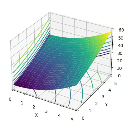
Shows how it behaves in the interval. Plotted above are the level sets in each plane. Most important for us, of course, are the level sets for ${x:f(x)=c}$, which is on the “xy” plane.

Visually, it is easy to see how [0,0] is the only minimizer. Below are the gradients plotted over the level set:

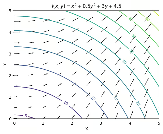
Notice that at any interior point, there exists a feasible direction that points away from the gradient, hence $\nabla f(x)<0$ and does not satisfy the FONC.

Point [0,0] on the other hand does. Let’s compute the gradient:

$$\nabla f(x)=\begin{bmatrix}2x_1\\x_2+3\end{bmatrix}$$

Because we are on the boundary, it does not suffice to say $\nabla f(x)=0$. Instead, we must have:

$$d^T\nabla f(x)\geq0 \ \forall \ d$$

At [0,0], $d^T\nabla f(x)$ is simply $3d_2$. However, for $d$ to be feasible we demand both $d_1, d_2\geq0$, so for sure $d^T\nabla f(x)\geq0$ at $x=[0,0]^T$.

Example: Second Order Necessary Condition

Consider the function:

$$f(x)=x^T\begin{bmatrix}2&5\\-1&1\end{bmatrix}x+x^T\begin{bmatrix}3\\4\end{bmatrix}+7$$

Let’s try to find minimizers! This function’s minimizers must satisfy the first and second order necessary conditions. Taking its gradient and Hessian yields:

$$\nabla f(x)=\begin{bmatrix}4x_1+4x_2+3\\4x_1+2x_2+4\end{bmatrix}$$ $$F(x)=\begin{bmatrix}4&4\\4&2\end{bmatrix}$$

To satisfy the FONC, we solve:

$$4x_1+4x_2+3=0, 4x_1+2x_2+4=0$$

Which yields the single point:

$$x=\begin{bmatrix}-5/4\\1/2\end{bmatrix}$$

Which is our suspect. Let’s use our definiteness tool for the Hessian to verify the second order necessary and sufficient conditions. From Sylvester’s Criterion:

$$\det (F_0)=4$$ $$\det(F_1)=\begin{vmatrix}4&4\\4&2\end{vmatrix}=8-16=-8$$

So the Hessian is neither positive definite nor positive semidefinite. In fact, it is indefinite. Because this fails the SONC, and it is the only point that could be a local minimizer (satisfies FONC,) the function does not have any minimizers. Sad day for $f(x)$.

Example: A bit of trouble!

Here’s an example where the FONC is a bit useless unless you rethink the problem a bit. Consider the problem of minimizing $f(x)$ in $\mathbb{R^2}$ subject to the following set constraint:

$$\Omega=\{x_1,x_2 \ | \ x_1^2+x_2^2=1\}$$

Let’s try to find minimizers. The FONC is:

$$d^T\nabla f(x)\geq0$$

For all feasible directions. However, there are no feasible directions in any x! Here’s why: The set is the edge of a unit circle. From any point in the circle, you cannot choose a direction where you remain on the edge along all points in the line you march. Sure, you can march towards another opposite edge. However, there would exist an $\alpha$ such that $x+\alpha d \notin \Omega$. This would correspond to an $\alpha$ that lands you inside the circle, not on the edge. You could also pick the tangent to the point where you are in. However, marching some small step along that tangent would put you very close but not quite on the edge.

Because of this, every single point in the set satisfies the FONC. Notice how the FONC here is not useful at all for narrowing down local minimizer candidates.

We can rephrase this problem, however. If we parametrize the points along $\Omega$ with:

$$x_1=\cos{\theta} \ \ \ \ \ x_2=\sin{\theta}$$

We can use the FONC with respect to $\theta$ instead. Now, $x=g(\theta)$, so we minimize the composite function $f(g(\theta))$. Its gradient by the chain rule is:

$$Df(g(\theta))\nabla g(\theta)$$

But $\nabla g(\theta)=[-\sin{\theta},\cos{\theta}]^T$. The FONC is now applied to $\theta$ instead!

Conclusion

Though I digressed a bit, the insight here is that tools from linear algebra that might seem irrelevant and simplistic pop up all the time in applications. I spared this post from a motivation into why this is all so important, but it is easy to see how applicable this is to engineering design optimization. Even the most simple devices can have unexpected optimization problems.

3Blue1Brown has a fantastic video on Newton’s Method and how Newton’s Fractal appears in it. He motivates the viewer with a computer graphics example: how can a point know whether it must be colored white or black if that decision is based off of its distance from a curve of known geometry? It is easy to see here that any point on the screen might want to solve the problem of minimizing the distance between its position and the curve.

Of course, a lot of the applications of the theories above are more in the field of numerical methods - questions such as how do you numerically compute the gradient and Hessians when their closed-form are not known - but the foundations are simple yet extremely insightful ideas as the ones shown above.

Anyways, hope you enjoyed it!